What is the average Rugby World Cup score?

September 1, 2023 - 3 mins read

Over the weekend, I started writing a rugby guide for newbies. In it I wanted to include some information about the average score of a RWC match. I thought it would be interesting to see how the average score has changed over time, and the difference between pool matches and knockout matches.

Thankfully, this requires a reasonable small dataset that is already available having worked on Rugby Bot for the past few years. This includes all Men’s matches from the World Cup until the 2019 edition.

print(df.shape)
>>> (377, 18)

and in true data science fashion, the data is the most important part. We need to remove the matches that were cancelled in the 2019 World Cup, otherwise these “0-0” matches will distort our averages.

df = df[~df.cancelled]
df.shape
>>> (374, 18)
df.columns
>>> Index(['id', 'c_home', 'c_away', 'dt', 'dt_utc', 'score_h', 'score_a',
       'venue_id', 'home_name', 'away_name', 'venue', 'm_pool', 'qf', 'sf',
       'bronze', 'final', 'knockout', 'cancelled'],
      dtype='object')

“Home” and “Away” don’t really apply in a World Cup context, so we can use more appropriate fields:

df["winner"] = df.apply(lambda x: x["c_home"] if x["score_h"] > x["score_a"] else x["c_away"], axis=1)
df["loser"] = df.apply(lambda x: x["c_home"] if x["score_h"] < x["score_a"] else x["c_away"], axis=1)
df["score_w"] = df.apply(lambda x: x["score_h"] if x["score_h"] > x["score_a"] else x["score_a"], axis=1)
df["score_l"] = df.apply(lambda x: x["score_a"] if x["score_h"] > x["score_a"] else x["score_h"], axis=1)

Now that we are set up, we can run some quick calculations:

df.score_w.mean(), df.score_l.mean(), (df.score_w - df.score_l).mean()
>>> (38.37433155080214, 12.885026737967914, 25.489304812834224)

Average Result

Overall, the average result in Rugby World Cup matches is 38 - 13. At first pass, these numbers seem higher than the usual matches in the Six Nations or Rugby Championship. This would be due to the fact that there is a bigger difference in rankings in the World Cup, and more one-sided matches.

Pools vs Knockouts

Let’s split it by pool and knockout matches:

df_pool = df[~df.knockout]
df_knockout = df[df.knockout]
df_pool.score_w.mean(), df_pool.score_l.mean(), (df_pool.score_w - df_pool.score_l).mean()
>>> (40.94039735099338, 12.6158940397351, 28.32450331125828)
df[df.knockout].score_w.mean(), df[df.knockout].score_l.mean(), (df[df.knockout].score_w - df[df.knockout].score_l).mean()
>>> (27.61111111111111, 14.01388888888889, 13.597222222222221)

So the pool matches are much more one sided than the knockout matches, as expected.

We can further break this down by stage of knockout match:

# Different knockout stages
stages = ["qf", "sf", "bronze", "final"]
stagedata = []
for stage in stages:
    df_stage = df[df[stage]]

    stagedata.append((stage, df_stage.score_w.mean(), df_stage.score_l.mean(), (df_stage.score_w - df_stage.score_l).mean()))

pd.DataFrame(stagedata, columns=["stage", "score_w", "score_l", "diff"])

	stage	score_w	score_l	diff
0	qf	30.611111	14.972222	15.638889
1	sf	25.055556	13.722222	11.333333
2	bronze	26.111111	13.888889	12.222222
3	final	22.222222	10.888889	11.333333

The scores get closer as we go further in the tournament. However, the bronze match and Final only have a sample size of 9 which is not a significant amount. But it does support our general intuition.

Across Tournaments

We can also have a look at how the scoring changes across tournaments:

# Across Tournaments
per_tournament = df.groupby(df.dt.str[0:4]).agg({"score_w": "mean", "score_l": "mean"})
per_tournament["diff"] = per_tournament.score_w - per_tournament.score_l

dt	score_w	score_l	diff
1987	37.5625	13.0938	24.4688
1991	27.5312	9.875	17.6562
1995	38.9375	15.125	23.8125
1999	43.3902	15.561	27.8293
2003	45.9583	13.375	32.5833
2007	39.2917	12.3333	26.9583
2011	35.75	11.0208	24.7292
2015	36.625	14.1875	22.4375
2019	37.2889	11.5111	25.7778

For knockouts only:

per_tournament_ko = df_knockout.groupby(df_knockout.dt.str[0:4]).agg({"score_w": "mean", "score_l": "mean"})
per_tournament_ko["diff"] = per_tournament_ko.score_w - per_tournament_ko.score_l

dt	score_w	score_l	diff
1987	30	12.125	17.875
1991	18.125	8.875	9.25
1995	31.125	17.875	13.25
1999	34	19.5	14.5
2003	29.875	13.75	16.125
2007	23.5	12.375	11.125
2011	17.875	10	7.875
2015	33.75	18.625	15.125
2019	30.25	13	17.25

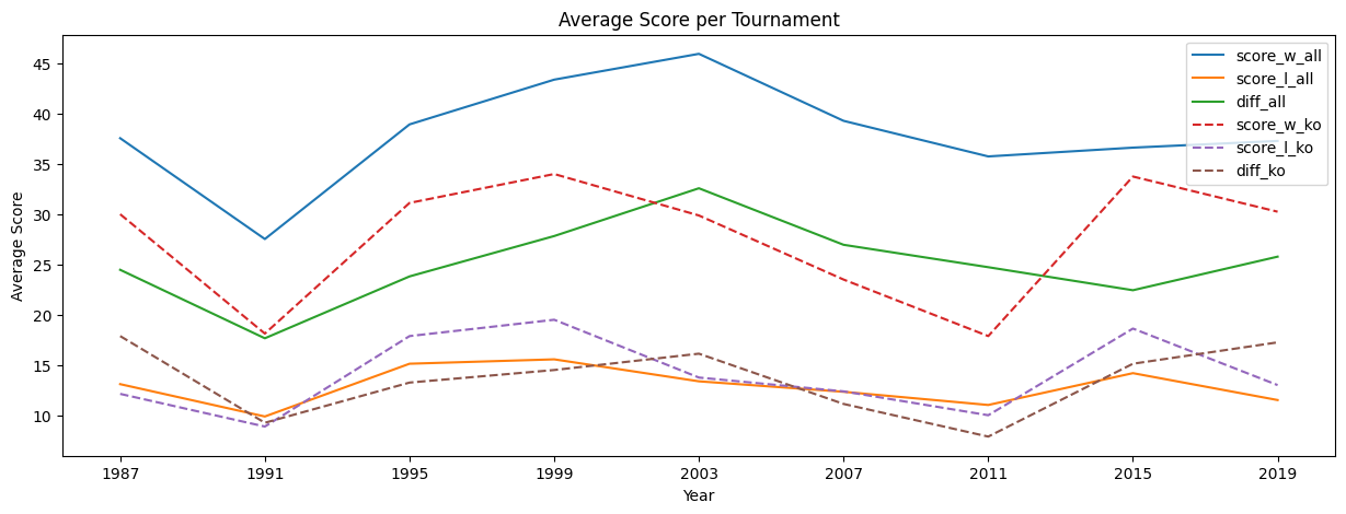
The knockout difference makes sense. Thinking back to the 2007 and 2011 World Cups, the knockout matches were quite … an arm wrestle (snore).

Graph

Since it’s likely easier, we can plot these results for a slightly easier view.

graph

What will the 2023 World Cup look like?